Most machine vision projects fail in the lighting, not the algorithm. If the defect does not change the pixels in a repeatable way, no amount of training data will make it reliable.
This guide is for the person who has been asked to “add camera inspection” to a line in India: what the physics allows, how to size resolution and lighting, when a classical rule beats a neural network, and how to write an acceptance test that decides whether the system is actually working.
Start with the defect, not the camera
Write down the defect in physical terms before shortlisting hardware. “Scratch” is not a specification. “A 0.3 mm wide bright line, at least 2 mm long, on a brushed aluminium surface, visible under low-angle light” is something you can design for and test against.
- Size: the smallest feature that must be detected, in millimetres.
- Contrast: how much the defect differs from good product in the chosen illumination.
- Variation: how much good product itself varies in colour, texture and position.
- Rate: parts per minute and the time window available for inspection.
- Consequence: what happens if you miss one, and what happens if you reject a good part.
The last two decide the whole architecture. A missed crack in a brake component and a false reject on a plastic cap have completely different economics, and the system should be designed differently for each.
Resolution arithmetic you can do on paper
Field of view divided by sensor pixels gives millimetres per pixel. A useful rule is at least three pixels across the smallest defect you must detect, and five is comfortable. Below three pixels, the defect is a single grey dot that noise can imitate.
# example: inspect a 120 mm wide part
fov_mm      = 120          # width the camera must see
sensor_px   = 2448         # horizontal pixels, 5 MP area scan
mm_per_px   = fov_mm / sensor_px        # 0.049 mm per pixel

smallest_defect_mm = 0.3
pixels_across = smallest_defect_mm / mm_per_px
print(round(pixels_across, 1))          # 6.1 px -> comfortable

# time budget per part
parts_per_minute = 60
cycle_ms = 60000 / parts_per_minute     # 1000 ms total, capture + process + reject
Two consequences follow immediately. Doubling the field of view halves the resolution, so a wide shot that covers the whole conveyor cannot also resolve a fine scratch. And a line scan camera changes the arithmetic entirely: resolution is set across the belt, and the scan rate is set by line speed.
| Camera type | Strength | Limit | Typical use |
|---|---|---|---|
| Area scan, global shutter | Simple, stops motion cleanly | Resolution falls as field of view grows | Stationary or indexed parts |
| Area scan, rolling shutter | Cheaper, higher resolution | Skew on moving parts | Static inspection only |
| Line scan | Very high resolution on a moving web | Needs encoder and uniform lighting | Sheet, film, cable, continuous strip |
| 3D profile sensor | Height and depth defects | Slower, more data | Weld beads, gaps, flushness |

Lighting does the heavy lifting
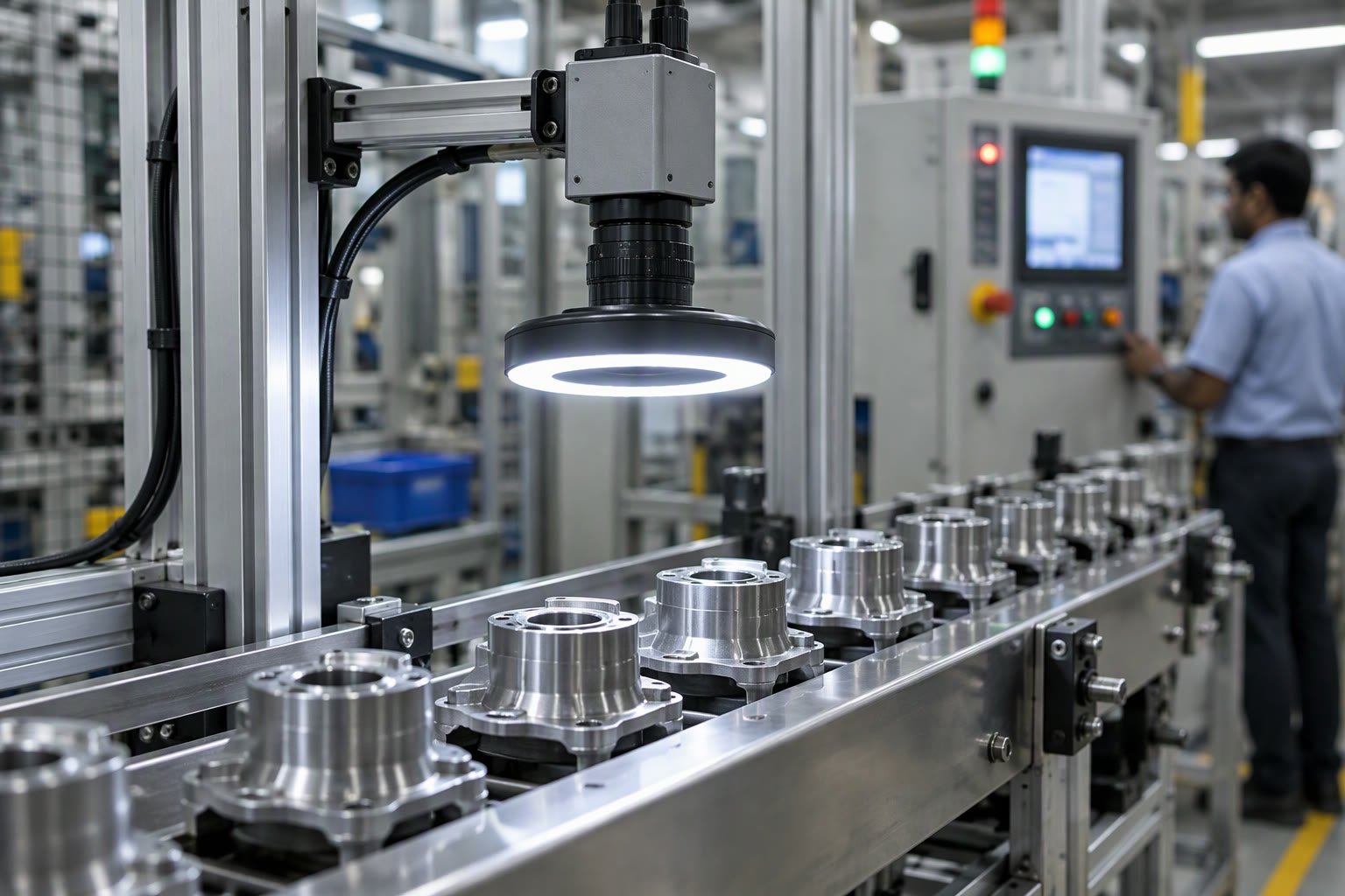
Lighting is where a ₹40,000 camera outperforms a ₹4,00,000 camera with bad illumination. The goal is not brightness; it is contrast that survives normal variation.
- Backlight — silhouette measurement. Excellent for holes, gaps and edge position, useless for surface defects.
- Low-angle dark field — rakes across the surface and makes scratches and dents glow. The standard choice for machined and brushed metal.
- Dome or diffuse — even light on curved, reflective parts. Removes hotspots on polished surfaces.
- Coaxial — light along the lens axis for flat, mirror-like surfaces and engraved marks.
- Colour and filters — a coloured light or bandpass filter can turn an invisible contrast difference into a strong one without changing hardware.
The machine vision lighting guide goes deeper on geometry and offers a worked selection process. The short version: buy the light before the camera, and test it on real parts at the real line speed.
Rules or deep learning
Classical inspection measures things: edges, blobs, grey-level statistics, template correlation. Deep learning classifies or segments what it has seen before. Neither is universally better.
| Approach | Works well when | Struggles when | Effort |
|---|---|---|---|
| Threshold and blob analysis | Defect is much brighter or darker than background | Texture varies between good parts | Low, explainable |
| Edge and measurement tools | You need a dimension or position | Defect is a surface flaw | Low, precise |
| Template matching | Part orientation is fixed and repeatable | Rotation, scale or lighting change | Low, brittle |
| Deep learning classifier | Defect appearance is complex but labelled data exists | Rare defect classes with few images | High, needs data |
| Anomaly detection | Only good parts are available | Subtle defects that look like good parts | Medium, unpredictable |
A practical default for a first project: solve it with rules if the defect has a clear physical signature, and only move to learning when the rules produce unacceptable false rejects. A rules-based system is easier to explain to a quality manager, which matters more than elegance during acceptance.
The data problem nobody budgets for
If you choose a learned model, the project becomes a data project. Plan for it honestly.
- Collect images across shifts, operators, material batches and lighting conditions, not one afternoon.
- Include the marginal cases. The system’s job is to decide on the hard ones, and those are exactly the images that get thrown away.
- Label with a written definition and a second reviewer. Two people disagreeing on what counts as a scratch is a specification problem, not an AI problem.
- Hold back a test set from a different day. A model that scores 99 percent on the same session it trained on has learned the session.
For deep learning on the edge, the Jetson Orin Nano setup guide covers building and benchmarking an inference engine, and YOLO object detection for robots explains training and deployment for detection rather than classification.
Integration: trigger, decide, reject, log
A vision system that only displays a result on a monitor is a demo. Production needs four connections.
- Trigger. A photoelectric sensor or an encoder position tells the camera when the part is in view. Free-running inspection without a trigger produces misaligned images and phantom defects.
- Decision. The result goes to a PLC as pass, fail or inconclusive, with a cycle-time stamp.
- Reject. A pneumatic pusher, a diverter or a robot pick removes the part. The reject mechanism must be tested with known-bad parts, not simulated ones.
- Log. Every image and result saved for a defined retention period. This is what lets you answer “why did we ship that” three weeks later.
The PLC handshake is usually the schedule risk, because the vision supplier and the line integrator each assume the other is handling it. The robot integration checklist lists the signals to agree in writing, and industrial Ethernet for robots explains the fieldbus options.
Indicative costs in India
Prices move with the rupee, import duty and camera availability, so treat these as planning bands rather than quotes. Get three written quotations for the same specification before committing.
| Element | Indicative range | Notes |
|---|---|---|
| Area scan camera, 5 MP, GigE | ₹35,000 to ₹1,20,000 | Global shutter and brand drive the upper end |
| Lens | ₹8,000 to ₹45,000 | Low distortion and fixed focal length cost more |
| Lighting and controller | ₹15,000 to ₹90,000 | Dome and coaxial are the expensive geometries |
| Industrial PC or edge computer | ₹60,000 to ₹2,50,000 | Depends on whether inference runs on GPU |
| Software licence | ₹0 to ₹4,00,000 | OpenCV is free; commercial suites are not |
| Integration and commissioning | ₹1,00,000 to ₹6,00,000 | Largest variable, driven by PLC work and reject hardware |
A single-station, rules-based inspection with a simple reject is often feasible at the lower end of these bands. Multi-camera, learned-defect systems with MES logging land far higher, and the integration line item is usually underestimated.
Write the acceptance test before you order
An acceptance test that says “detects defects” is unenforceable. Define the sample instead.
- 50 known-good parts from at least three production batches.
- 30 known-bad parts covering every defect class, with the defect location recorded.
- Ten marginal parts, agreed in advance as either pass or fail.
- Targets: escape rate and false reject rate, both stated as numbers, measured over the full sample at production speed.
- Repeat the run on a second day. If the result changes materially, the system is not stable.
Run the same test after any lighting change, lens change or model update. The test set becomes the regression suite, and without it every future tweak is a guess.
Questions to ask a supplier
- “Show me a system running on a similar part, in production, that I can call.” A reference video is not a reference.
- “What is the false reject rate you achieved, and who measured it?” Vague answers mean it was never measured.
- “What happens when the lighting drifts or a lens gets dusty?” A system without drift monitoring will fail silently.
- “Who owns the model and the images?” If you cannot retrain without the supplier, you have a subscription, not an asset.
- “What is the mean time to recover after a camera fault?” Downtime cost usually exceeds the hardware cost.
If the application also needs the robot to pick the part it inspected, the two projects should be scoped together. The vision guided robotics guide covers the hand-eye calibration and timing issues, and camera calibration in OpenCV is the prerequisite for any measurement in millimetres.
How many megapixels do I need for defect detection?
Work backwards from the smallest defect and the field of view. Aim for at least three pixels across the defect, five if the contrast is low. A 5 MP camera inspecting a 120 mm wide part gives about 0.05 mm per pixel.
Can I use a normal USB webcam for industrial inspection?
For a prototype on stationary parts, yes. For production, no: rolling shutter, auto-exposure, plastic lenses and no hardware trigger make results unrepeatable.
Is deep learning always better than classical vision?
No. Rules are more predictable, easier to explain and need no training data. Use learning when defect appearance is genuinely complex and you can collect labelled images across real production variation.
How much does a machine vision inspection system cost in India?
A single-station rules-based system typically starts in the low lakhs including camera, lens, light, PC and integration. Multi-camera or learned-defect systems cost substantially more, and integration is usually the largest line item.
Why does my inspection system pass good parts on the bench and fail them on the line?
Vibration, ambient light, part position variation and line speed all change the image. Commission and test at production speed with production parts, and lock the enclosure against ambient light.
For high-speed inspection, bandwidth decides whether the camera can keep up, so start with the interface comparison rather than the megapixel count.
A defect smaller than three pixels cannot be detected reliably, and the lens guide shows how to check pixels per millimetre before quoting.
If you are already inspecting parts, the OCR and code reading guide shows how to add traceability on the same camera.
Food grading is a high-variance vision problem, covered from the cell side in the food industry robot guide.
Inspection vision and bin-picking vision solve different problems and rarely share hardware.
Sources and further reading
- OpenCV documentation — image processing, calibration and classical inspection tools.
- A3 Association for Advancing Automation — machine vision standards and application notes.
- Basler camera documentation — sensor, shutter and interface specifications.
- Cognex vision resources — lighting geometry and inspection application guides.